Attention and transformers diagrams
Atlas of Stochastic Parrot Anatomy
Published:
Updated:
Some diagrams about attention in artificial neural networks and transformers architectures (as used in LLMs, vision transformers, VLMs).
Table of content
- Table of content
- Introduction
- Transformer encoder/decoder
- Encoder-only Transformer LLMs
- Decoder-only Transformer LLMs
- Attention
- Positional encoding
- FFN
- Additional sub-blocks
- Speculative decoding
- Perceiver
- Visual Transformers
- Detection
- Segmentation
- VLM
- Decision models
- Appendix, mathematical formulas
- Appendix, diagram notations
- References
Introduction
These diagrams were made by reading the papers describing the models and often cross-referencing the source code. In many cases, I found that the paper give a really high-level overview of the design/architecture but lacks a really detailed description of the architecture: key elements are peppered in the experimental result (as prose), buried in appendices, or completely absent from the paper and must be painfully recovered from the reference implementation. In several instances, I thought I had understood the architecture properly only to find out by reading a follow-up paper that I had missed some important detail.
Useful references:
- A Mathematical Framework for Transformer Circuits
- The Annotated Transformer
- LLM Architecture Gallery
- Transformers explained
- The Illustrated Trasnformer
Note: diagram reuse
These diagrams are released as CC0 (“No Rights Reserved”). Feel free to reuse/adapt these diagrams with attribution.
These diagrams are made with Ditaa. You can get the source of each diagram by replacing the .png extension with .ditaa.
Ditaa diagrams are much easier to modify and tweak than the previous versions (hand crafted SVGs). Moreover the source files can be used as plain ASCII art diagrams, which might be useful in some contexts. I can't really align the texts as I would like though.
Transformer encoder/decoder
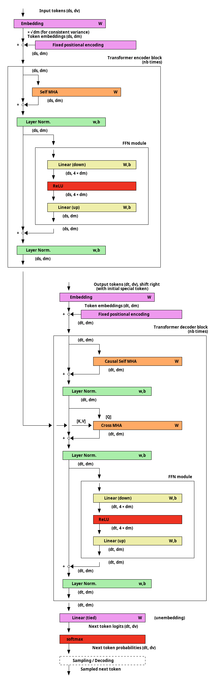
The original (encoder-decoder) Transformer architecture features separate input text and output text which are processed by the decoder and encoder respectively. The decoder uses (unmasked) self-attention and produce final token embeddings. The encoder uses both self-attention (often masked/causal) and cross attention (to the output of the final encoder block).
Encoder-only Transformer LLMs
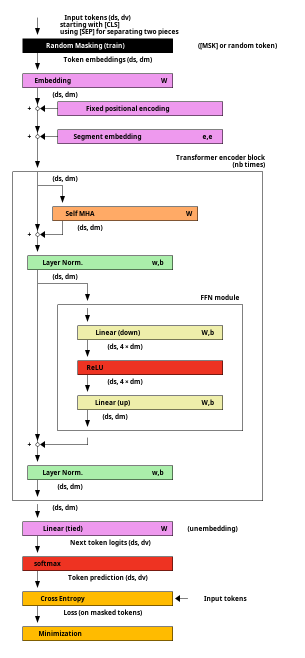
This diagram depicts one the two pre-training tasks of BERT (Masked Language Model): some tokens are masked and the model must predict them.
Decoder-only Transformer LLMs
GPT-1
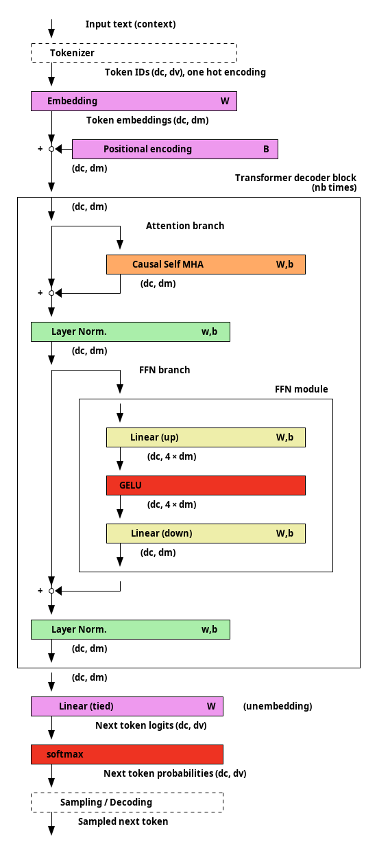
In contrast to subsequent models, it uses Post-Norm (the LayerNorm is after the residual branch instead of being at the beginning of the residual branch).
GPT-2
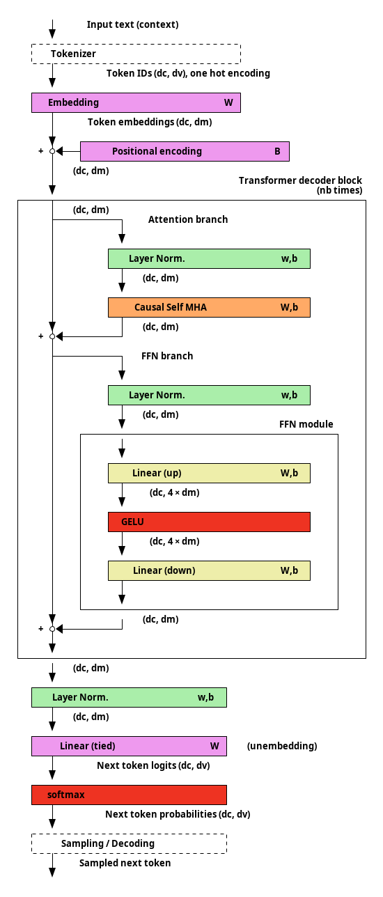
Llama 3
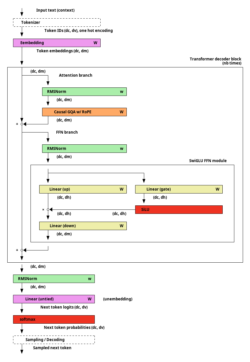
LLama 3 is an example of a typical “modern” LLM. Compared to GPT-2, it uses RMSNorm instead of LayerNorm, GQA instead of MHA, RoPE instead of learned positional encoding, a SiLU FFN, untied weights for token unembedding and does not use biases.
Attention
Attention operation
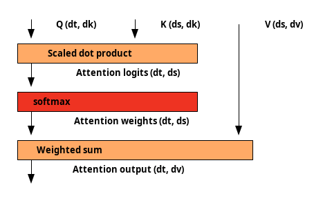
The
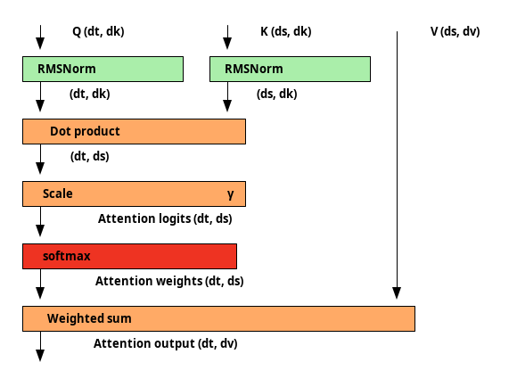
Dot-product attention with QK norm is actually cosine attention with a learnable temperature parameter.
SHA
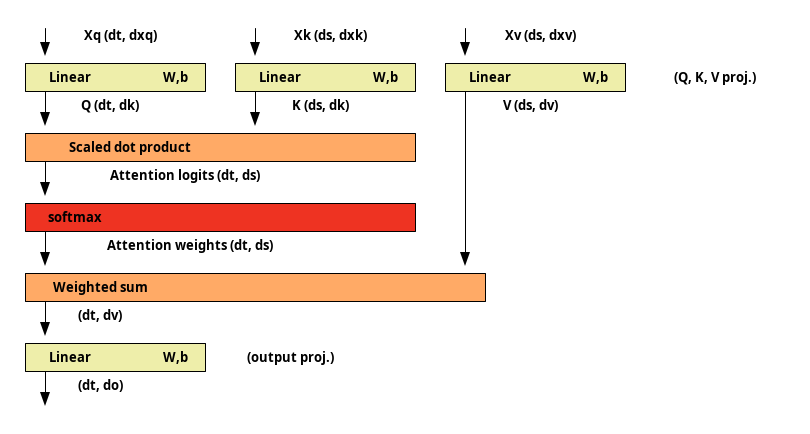
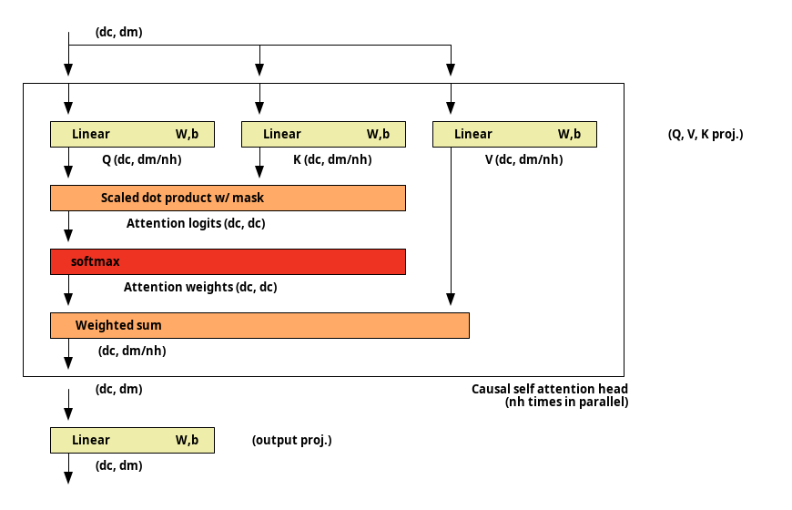
An typical attention module, includes projections for the query (Q), keys (K) and values (V) as well as an output projection.
MHA
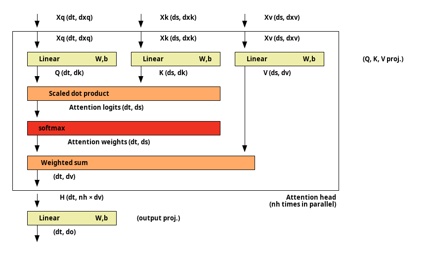
With MHA, the attention is split between different attention heads. Each attention head can attend to different aspects of the tokens. A conventional design uses
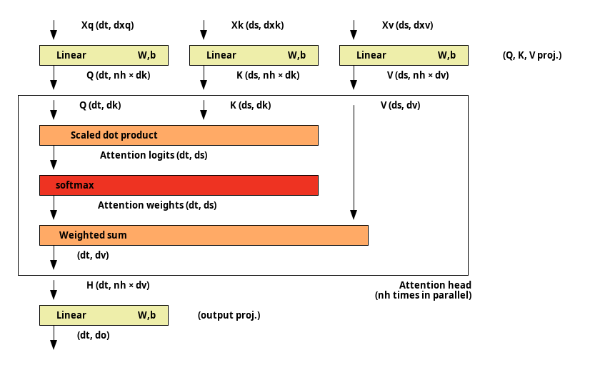
The previous diagram represents per head QKV projections (
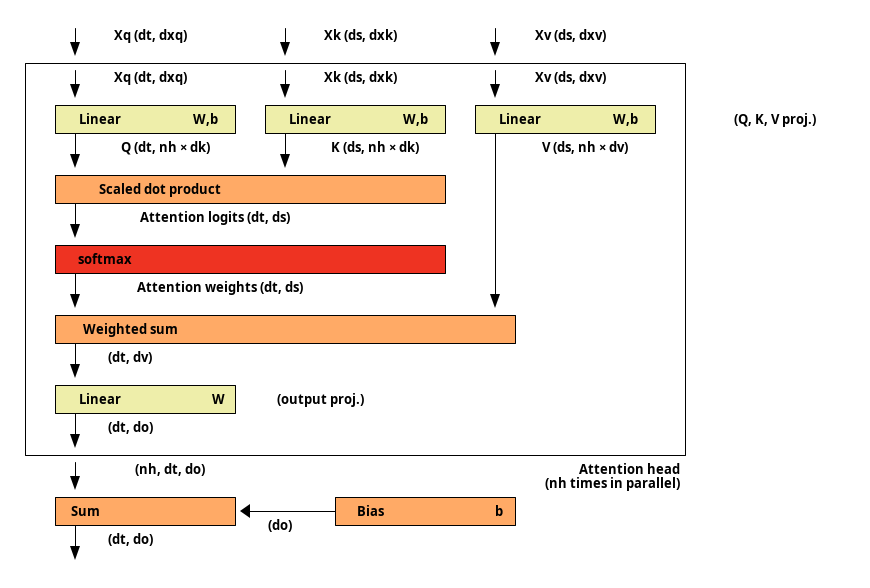
MHA can (equivalently) be understood as having per head output projections. When used in a residual structure, each attention head output projection is added to the residual stream (
MQA
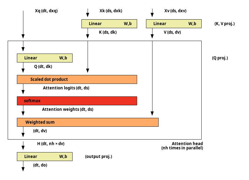
MQA reduces the size of the KV cache by using the same K and V for all attention heads.
GQA
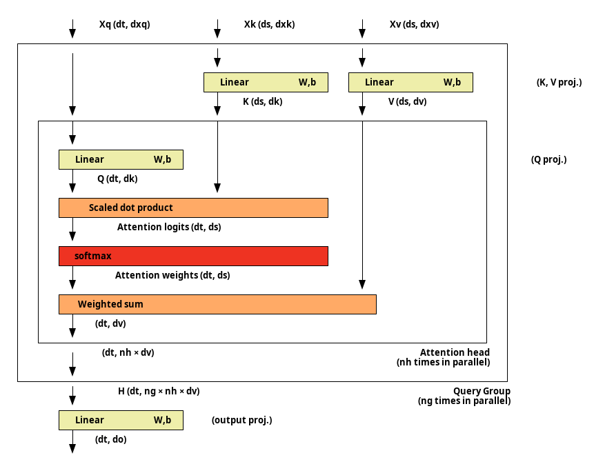
GQA is an intermediate between MHA (
MLA
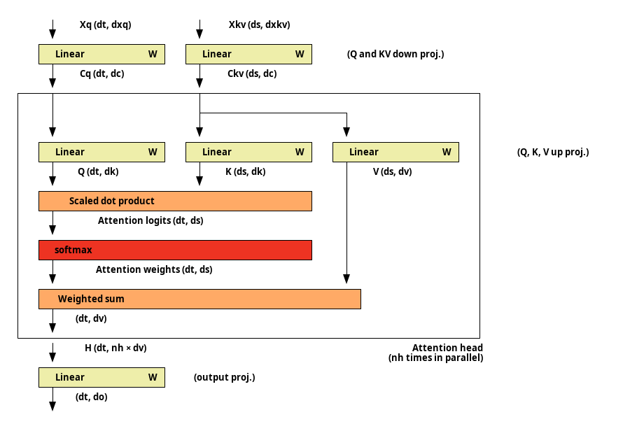
In MLA, a shared compressed latent representation of both keys and values (
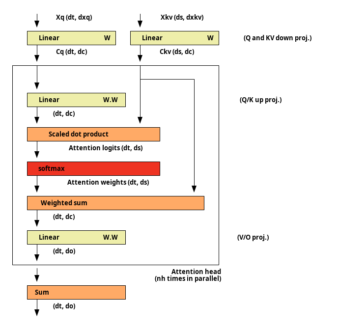
Through some linear algebra manipulations, we can do the operations in the compressed latent space.
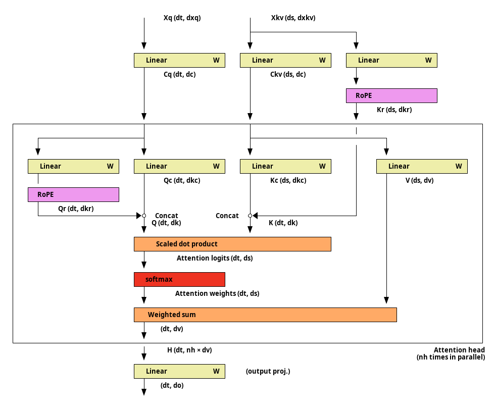
Query (
Sparse attention
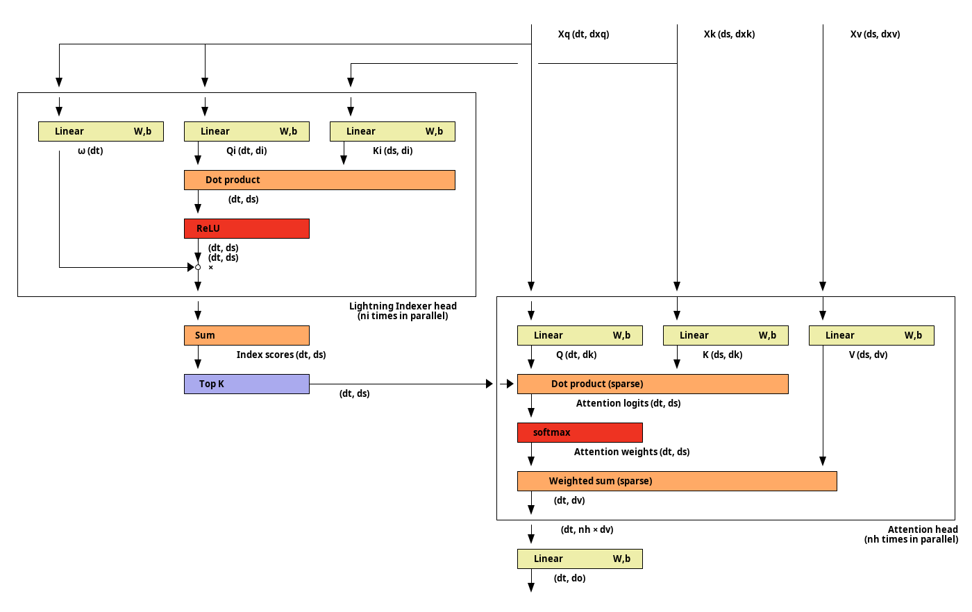
DSA uses a indexer heads to select K positions (Top K) to attend to for a given position (sparse attention). Here DSA is instanciated on top of MHA for simplicity.
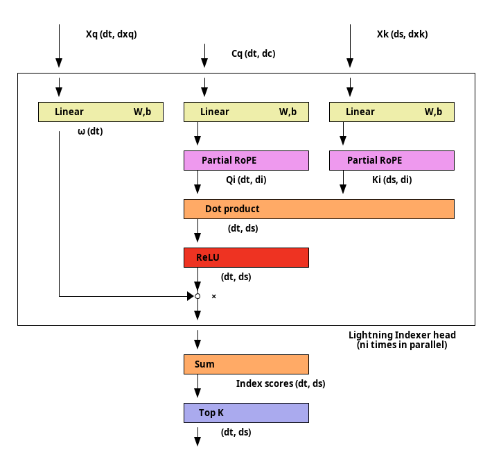
The DSA paper instantiates DSA on top of MLA with RoPE. This diagram show how RoPE is integrated into the DSA indexer.
Self-attention
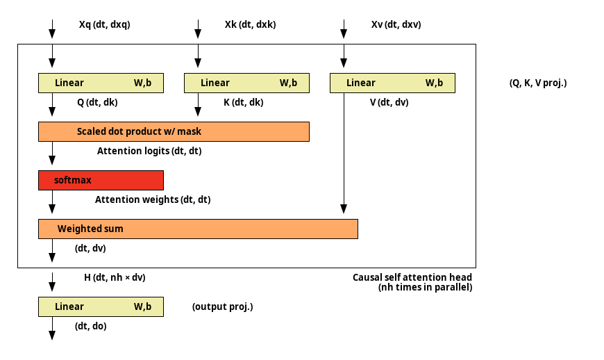
In self-attention, the source sequence and the target sequence are the same (and therefore
Deformable attention
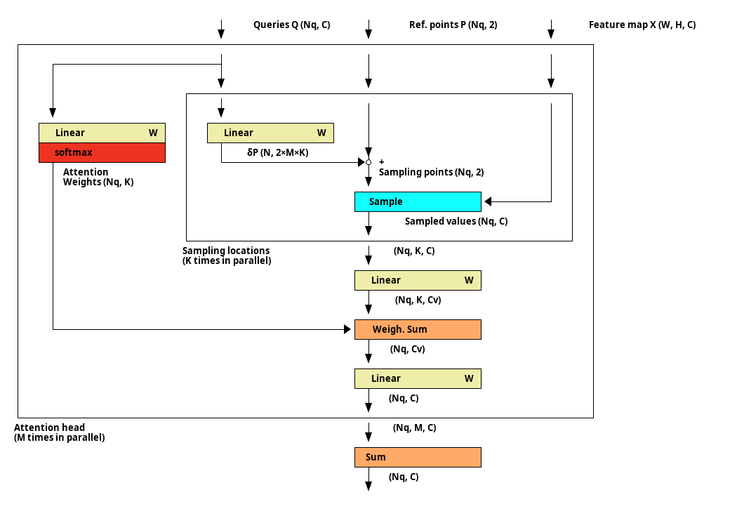
Deformable DETR uses deformable attention. For each query, each attention heads attends to a restricted number (K) of sampling positions of a feature map. Both the sampling positions and the attention weights are learned projections of the query.
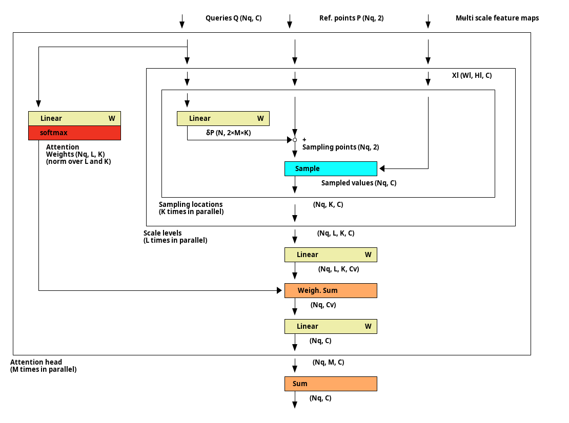
Multi-scale Deformable attention module extends Deformable attention with support for multi-scale feature maps. For each query, each attention head attends to K sampling position per scale level.
Positional encoding
RPB
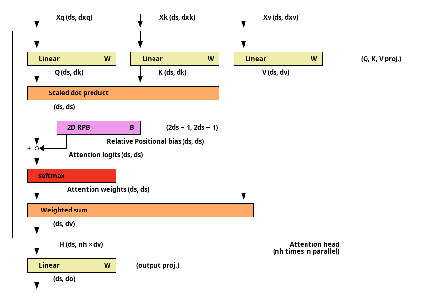
In RPB, learned (or fixed) positional encoding is adding to the attention scores (before the softmax). These biases depend on the relative position of the tokens.
Q/K positional encoding
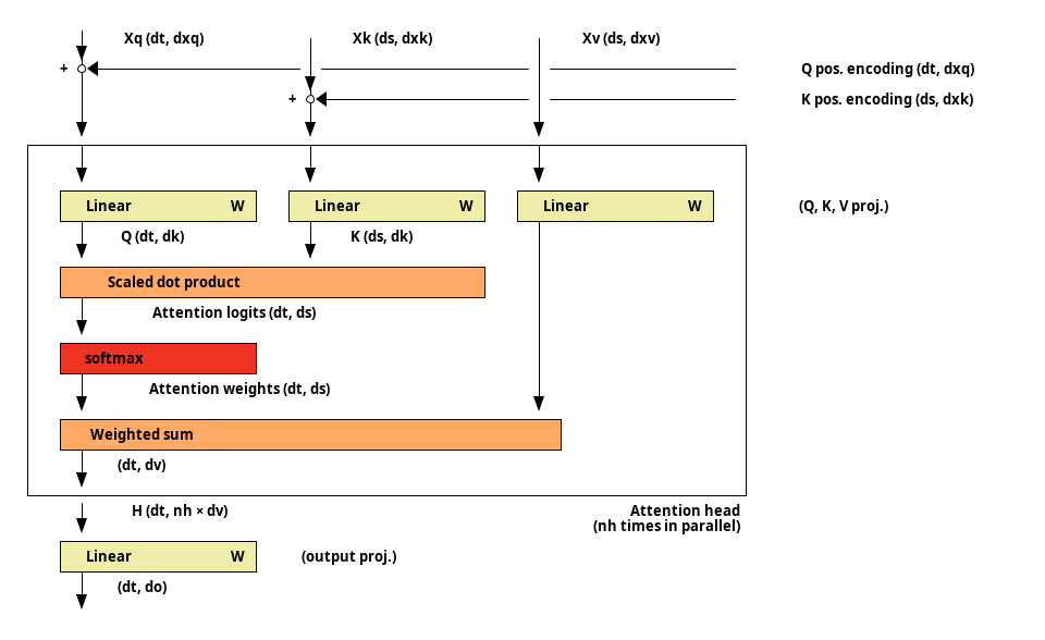
In this scheme, (learned or fixed) positional encoding is added before Q and K projection. The same positional encoding is used for all attention heads and for all attention blocks. For self-attention, the same positional embeddings are used for Q and K projections.
RoPE
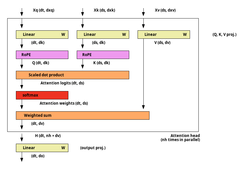
When using RoPE, the positional information is typically included in the Q and K of each attention block. The positional information is encoded by applying 2D rotations to pairs of features at different frequencies.
FFN
This sections compares different FFN modules.
Monolithic FFN
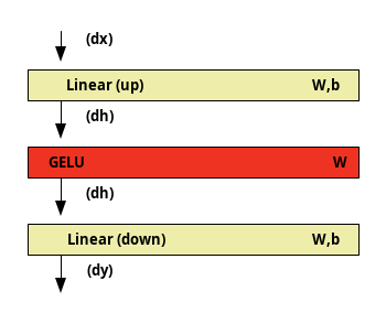
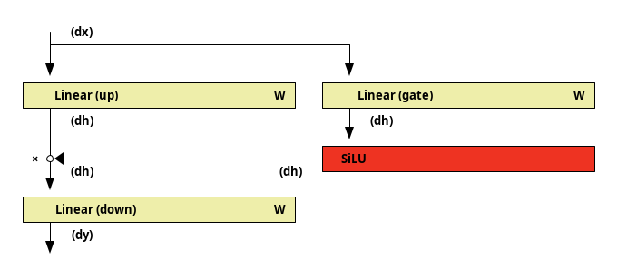
A typical design uses
Mixture of Experts
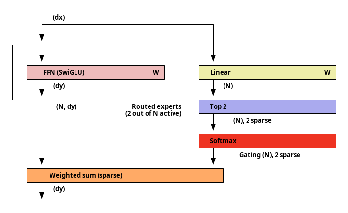
Mixtral replaces the FFN with sparsely-gated Mixture of Experts (MoE) where only two experts are active for each token (top 2).
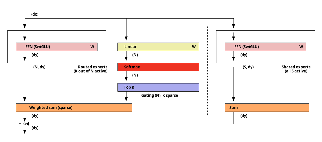
DeepSeekMoE replaces the FFN with sparsely-gated Mixture of Experts (MoE) where only K experts out of N are active for each token (top K). In addition, they include a small number of “shard experts“ which are always active (and are not gated).
Note: Evolution of MoE design in following DeepSeek versions
In DeepSeek V2, the n_routed_experts routed experts are distributed on n_group groups/devices (with n_routed_experts/n_group experts each). A first selection of topk_group devices is done and a total of num_experts_per_tok experts is selected among the (topk_group×n_routed_experts/n_group) experts of the selected groups.
In DeepSeek V3, the gating uses a sigmoid activation function (normalized) instead of softmax.
In DeepSeek V4, the gating uses sqrt(softplus(.)).
Additional sub-blocks
PLE
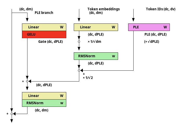
Gemma 4 uses per-layer token embedding (PLE). It is included through an additional gated residual sub-block at the end of the transformer block. This (comparatively-)small-dimension per-layer token embedding is combined with a down projection of the global token embedding.
Speculative decoding
MTP
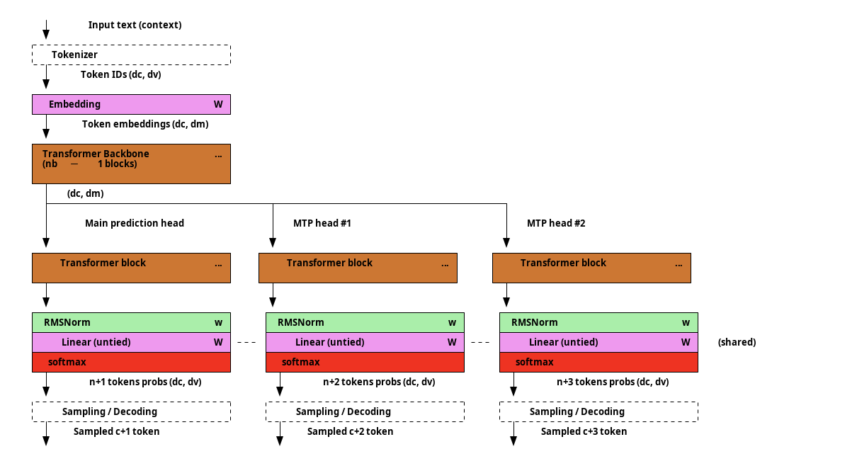
The original MTP design forks several independent prediction heads before the last transformer block, predicting respectively tokens at position n+1, n+2, etc.
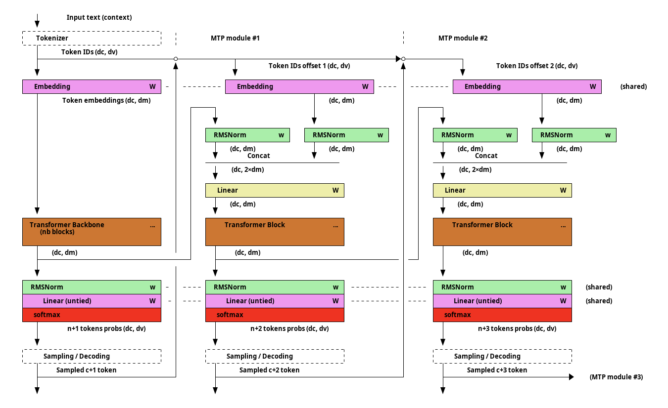
DeepSeek-V2 uses a chained MTP. The MTP prediction for token at position n+k uses the sampled tokens at positions n+1 to n+1-k.
EAGLE
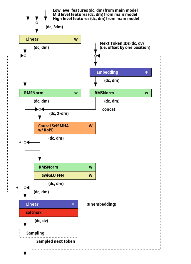
EAGLE-3 is an auto-regressive draft model. It takes as input the hidden features of the main model at three different levels and the token embeddings.
Perceiver
Vanilla Perceiver
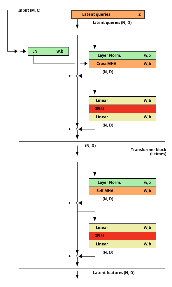
The Perceiver pattern can be used to handle large input sequences. It mitigates the quadratic complexity (wrt. sequence length
Perceiver IO
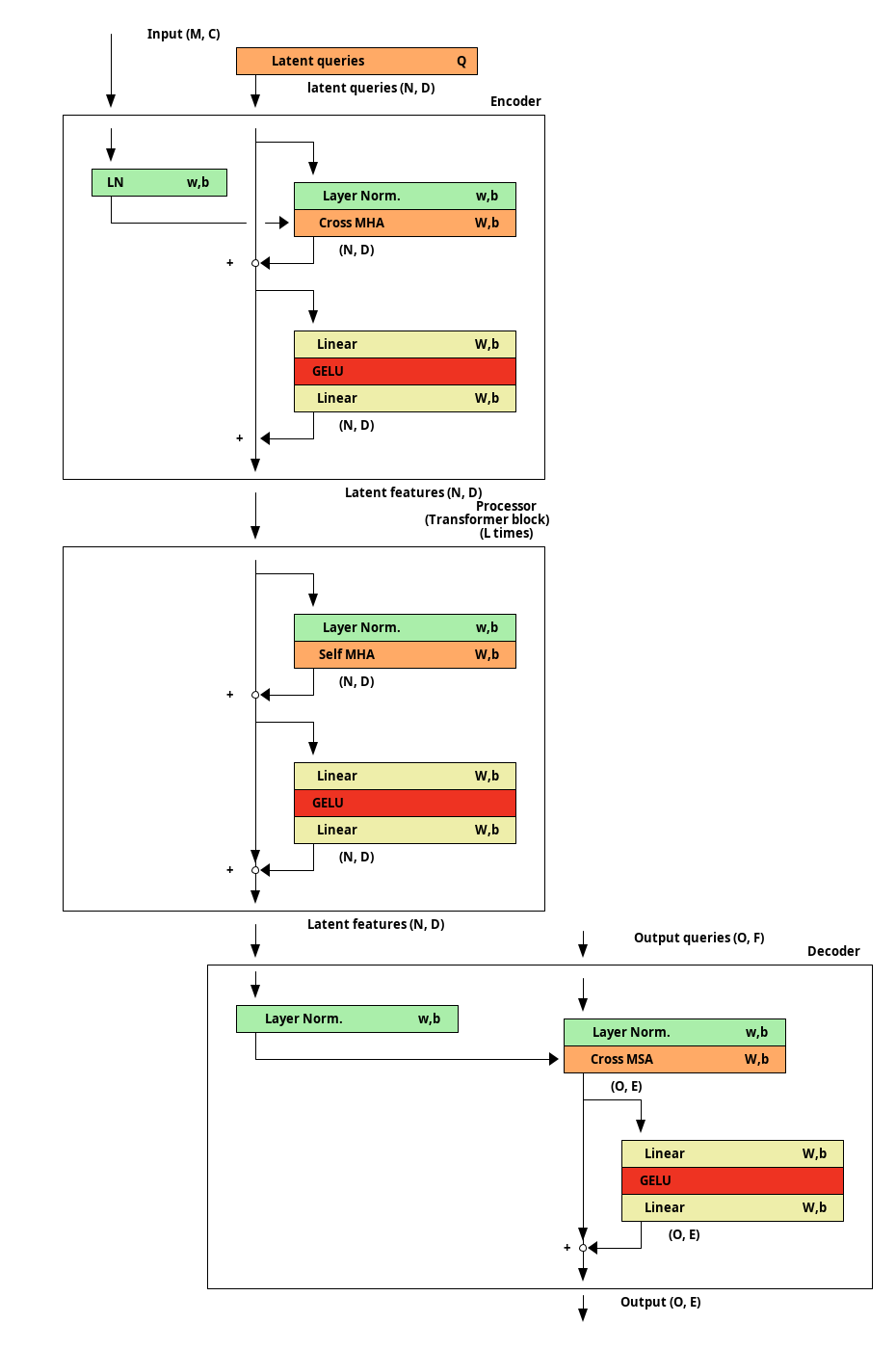
Perceiver IO adds another cross-attention block (decoder) where output queries attend to the latent features. For simple tasks, the output queries can be learned. For other tasks, the output queries can contains features describing the “task”. It is usually better to omit the skip connection around the output cross-attention (as depicted here) in this case.
Perceiver Resampler
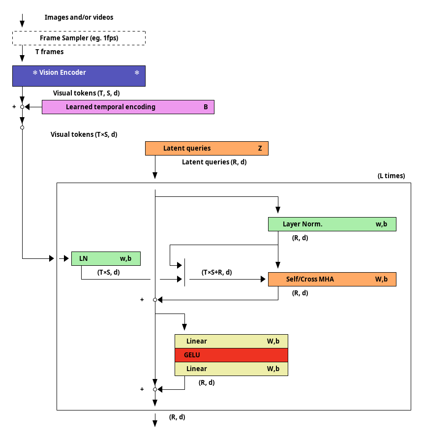
The Perceiver Resampler uses a Perceiver architecture to downscale a high number of visual token (eg. coming from a video) into a fixed number (R) of visual tokens. R latent queries attend to the visual tokens and to themselves in a mixed self/cross-attention operation.
Visual Transformers
ViT
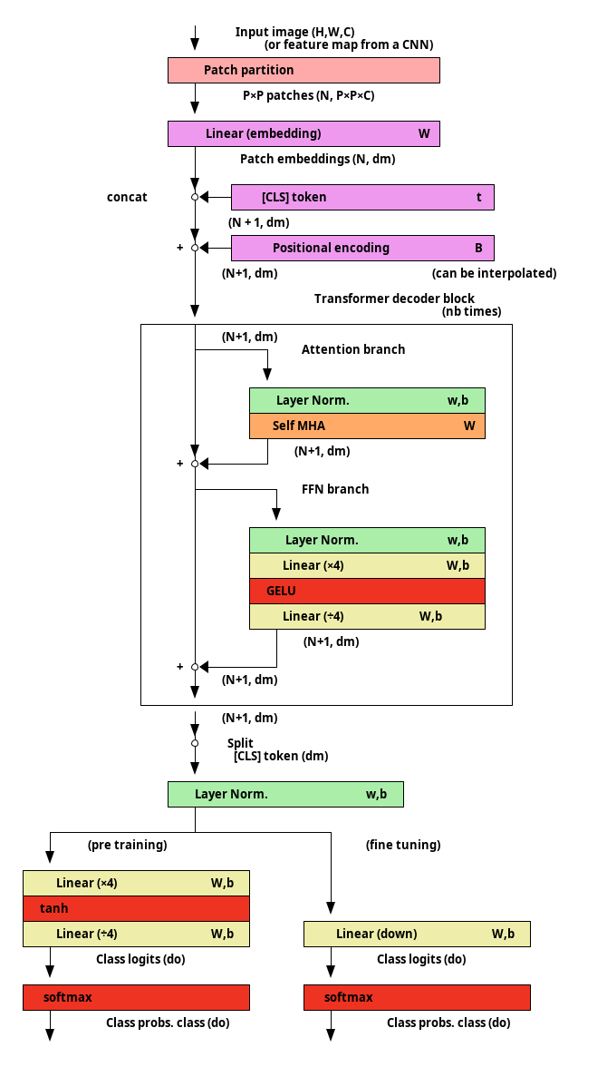
The input image is partitioned into (non-overlapping) patches of P×P pixels. These patches are seen as a sequence of tokens: each patch is first projected in the model embedding space and the resulting patch tokens are processed using a classic transformer decoder model. A special learned class token ([CLS]) is inserted at the beginning of the sequence: the final features of this token are fed into a classification head.
DeiT
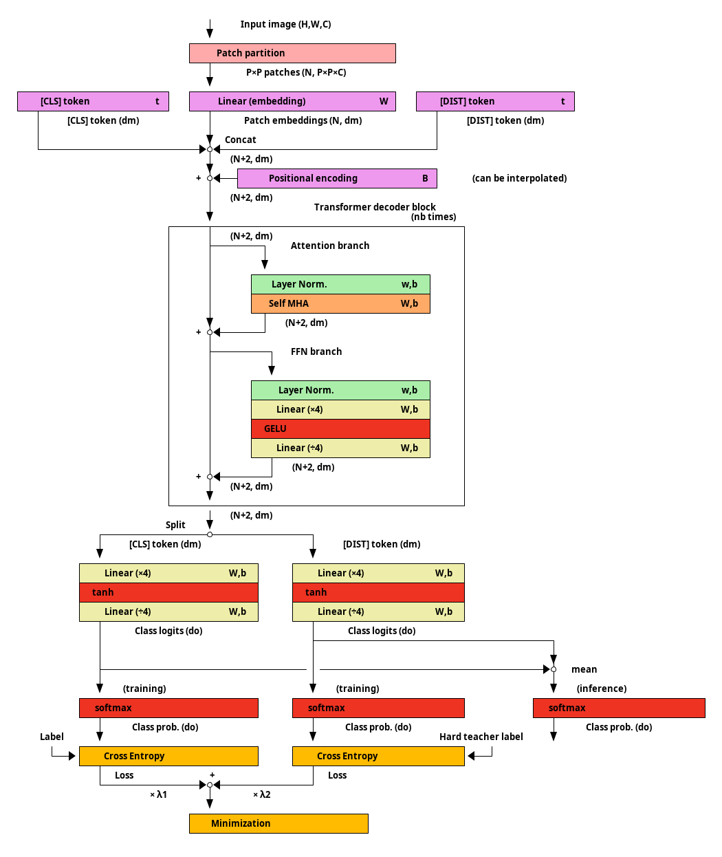
DeiT follows the architecture of ViT modified for the efficient distillation from a teacher model (eg. a ConvNet). An additional learned distillation token ([DIST]) is introduced. The student model is trained to match the teacher's predicted class through the distillation token (hard-label distillation), while simultaneously tracking the ground truth label through the class model.
At inference, the reference source code takes the mean of the logits of both heads.
Swin
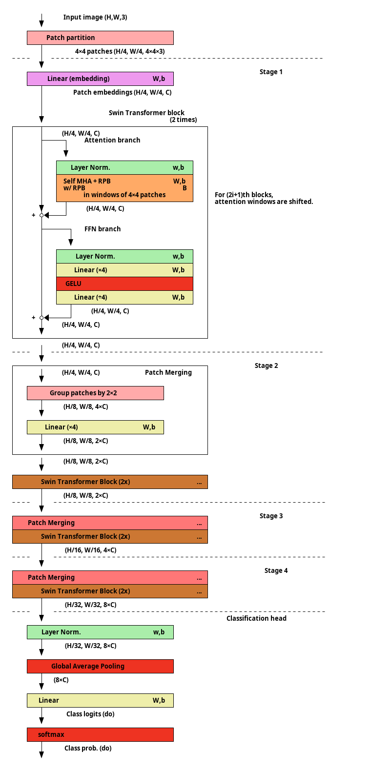
Swin encourages some form of locality by restricting the attention within windows of 4×4 patches and by using a hierarchical structure (patch merging). It produces a pyramid of multi-scale feature maps.
MAE
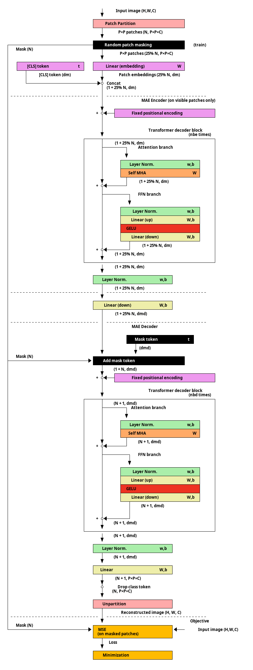
MAE (Masked autoencoders) uses self-supervised (pre-)training using an autoencoder network. The input image is severely degraded by masking a large proportion of patches. The masked patches are omitted from the sequence in the encoder and replaced by a learned masked token in the decoder. The network is trained must reconstruct the masked patches.
DINO
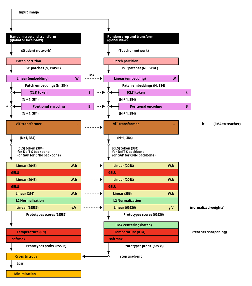
DINO (Distillation with no labels) uses self-supervised learning method through self-distillation (for pre-training). A student network is trained to follow the output of a teacher model (distillation). The student and the teacher receive a different “part” (crop/transformation) of the same image and produce a probability distribution in a high-dimensional “prototype” space. The student is trained to produce prototype distribution similar to the the distribution produced by the teacher, even if has received a different view of the same image. This forces the network to extract semantic information out of the image. The trick is that the teacher network is derived from previous version of the student network (self-distillation).
Notice the usage of weight normalization (torch.nn.utils.weight_norm, torch.nn.utils.parametrizations.weight_norm) in the output layer.
DINOv2
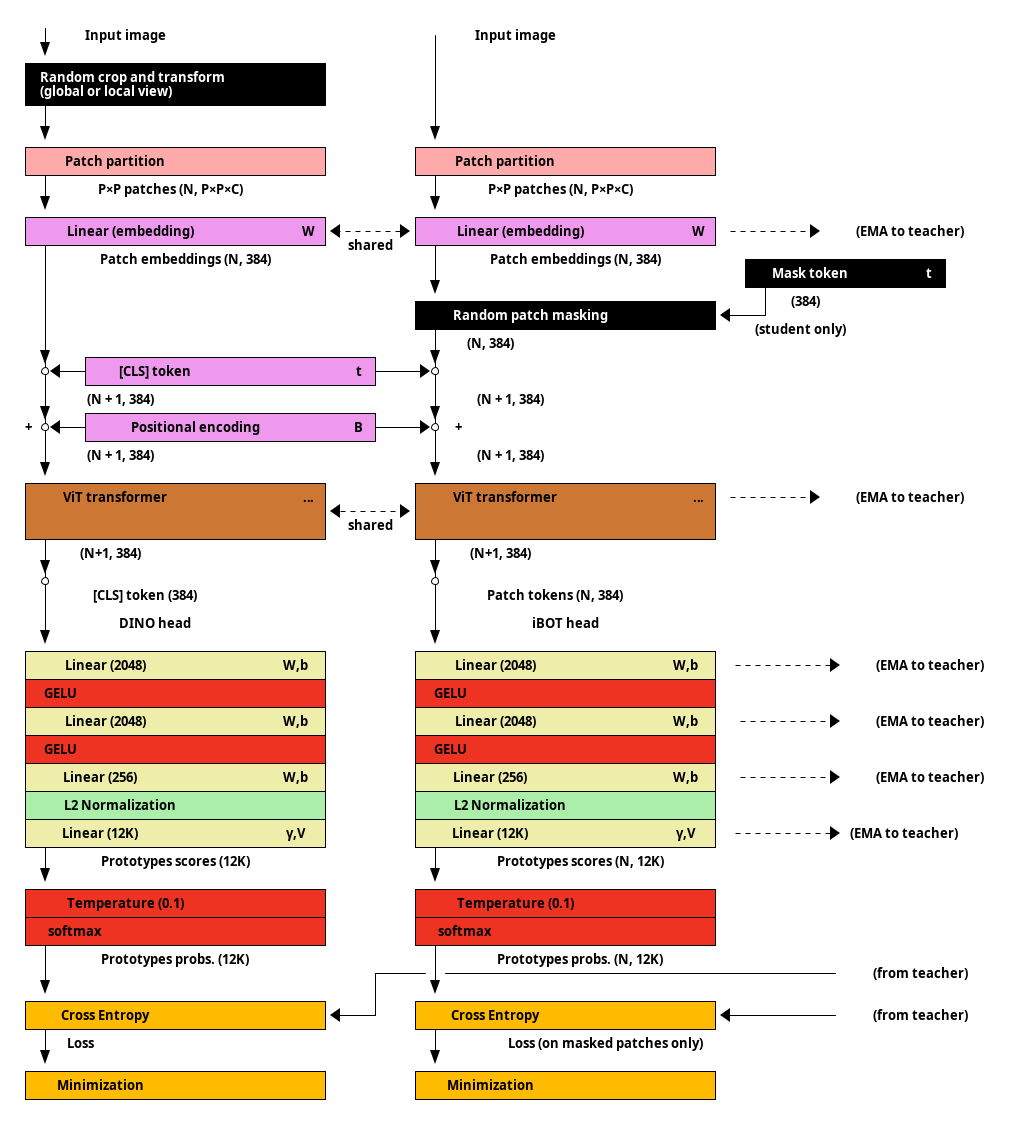
DINOv2 use the same style of self-distillation training as DINO but adds an iBOT-style objective. An additional head (the iBOT head) with the same architecture is added to the network. The second student head processes images where some patch tokens have been masked: it must learn to reproduce the prototypes produced by the teacher network (with unmasked data) for these masked patches.
The teacher network is not displayed in this diagram.
Detection
DETR
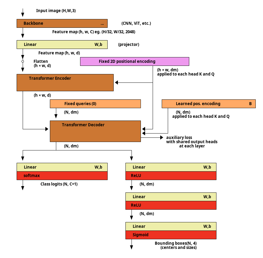
DETR is a transformer-based detection head which can plugged to an existing visual backbone (such as a ViT or a CNN). Compared to other detection heads, it does not requires Non Max Suppression (NMS) on the resulting bounding boxes because it is trained to avoid creating duplicate detections.
Deformable DETR
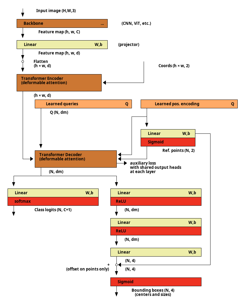
Deformable DETR but replaces the MHA in the encoder self-attention and the decoder cross-attention with multi-head Deformable attention modules. A variant, not depicted here use mutli-scale deformable attention (attending to multi-scale feature maps).
Some variants (not depicted here) mentioned in the paper are:
- multi-scale feature maps;
- iterative bounding box refinements;
- two-stage deformable DETR.
Segmentation
Maskformer
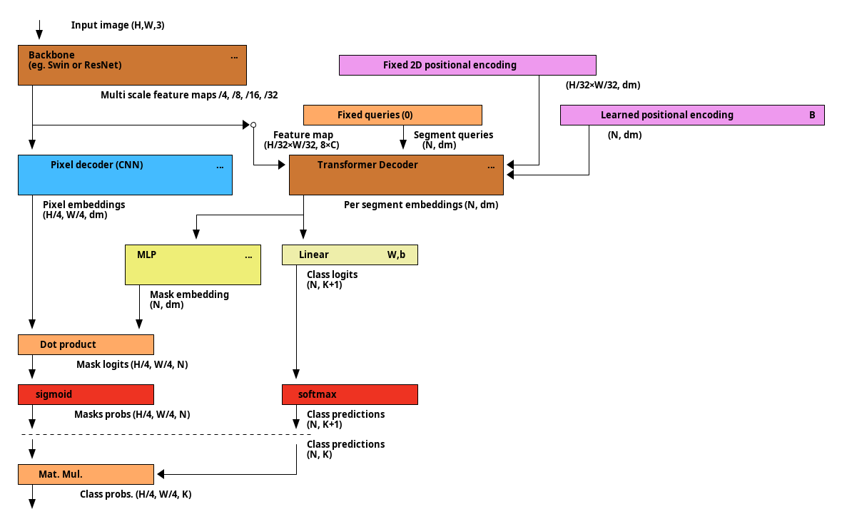
Maskformer uses a multi-scale backbone (/4, /8, /16, /32). The multi-scale feature maps are fed into a pixel decoder (FPN-like CNN) which produce final pixel embeddings as /4 scale. A transformer decoder uses fixed segment queries which attends to the low-resolution feature map (/32). The output of the transformer decoder is fed into two heads in order to produce two outputs. First, a classification head produces class prediction (classification) for each candidate mask/segment. Second, a MLP is used to produce per-mask embeddings for each segment query: the spatial masks (logits) are obtained by matching (dot product) the per-mask embeddings produced by the MLP with the pixel embeddings produced by the pixel decoder.
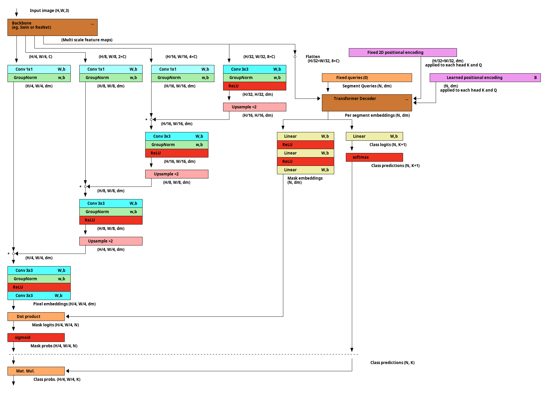
This diagrams details the FPN-like pixel decoder.
VLM
CLIP
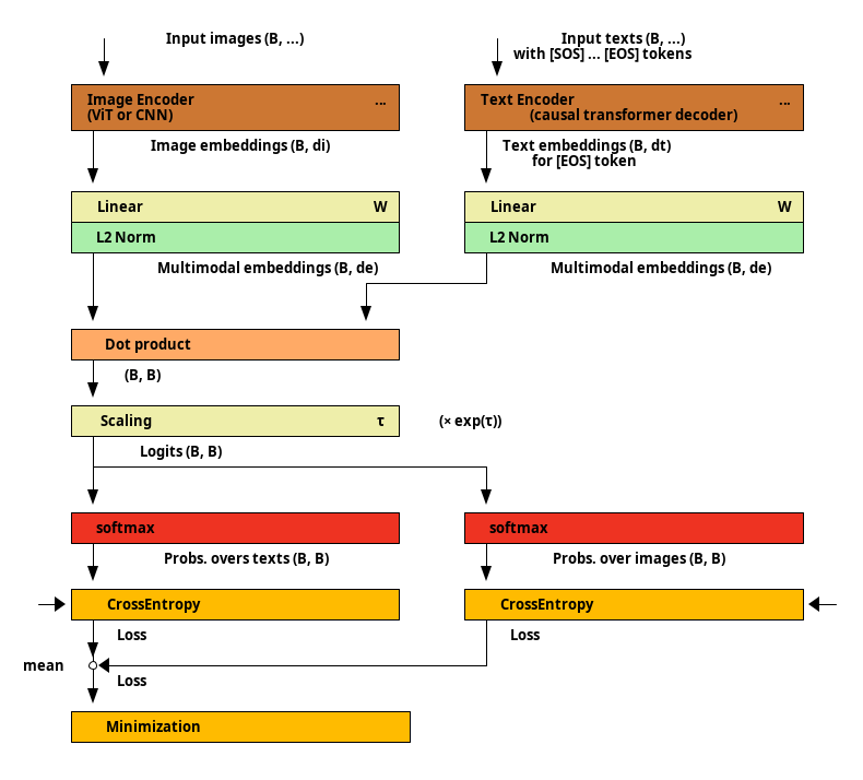
In CLIP (Contrastive Language–Image Pre-training), is trained using cross-modal contrastive learning. A visual model and a text models are jointly pre-trained using pairs (image, label) pairs. For each batch of B (image, label) pairs, the output of the visual encoder (a ViT or CNN) and the text encoder (an auto-regressive transformer decode model) are projected into a shared multi-modal embedding space. The model is trained to maximize the similarity of the representations of matching images and labels (and minimize the similarity of the representations of unmatched images and labels).
See SigLIP for an alternative (simpler) loss function.
BLIP-2
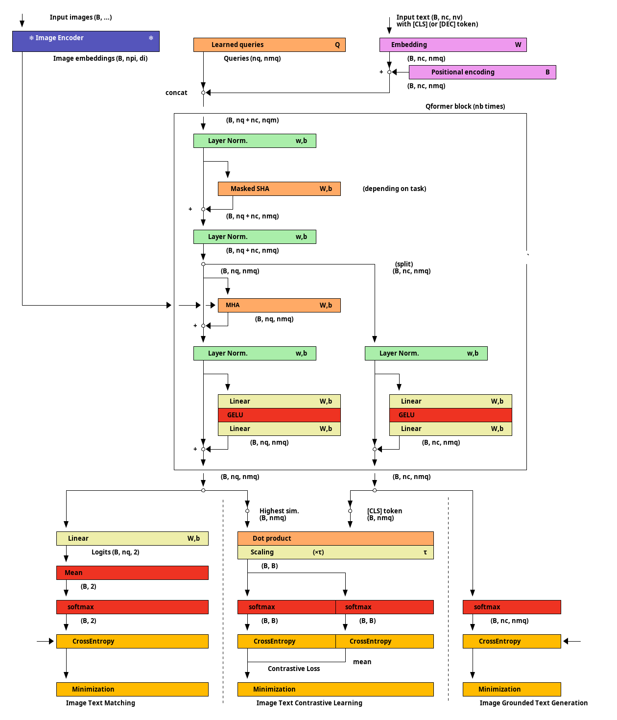
In the first stage of pre-training, the Qformer (Querying Transformer) learns to extract useful information from the output of frozen image decoder. The Qformer is initialized from an pre-trained LLM transformer (here BERT).
| Image Text Matching | Image Text Contrastive Learning | Image Grounded Text Generation | |
|---|---|---|---|
| Input | (image, text) pairs (true and false matches) | Batches of matching (image, text) pairs | Batches of (image, text) pairs |
| Goal | Binary classification (true/false ma tch) | Similarity for matching (image, pairs) | Maximize text probability |
| Self attention mask | None | Blocked between text and images | Multimodal causal |
| Mask, query → query | allowed | allowed | allowed |
| Mask, query → text | allowed | blocked | blocked |
| Mask, text → query | allowed | blocked | allowed |
| Mask, text → text | allowed | allowed | causal |
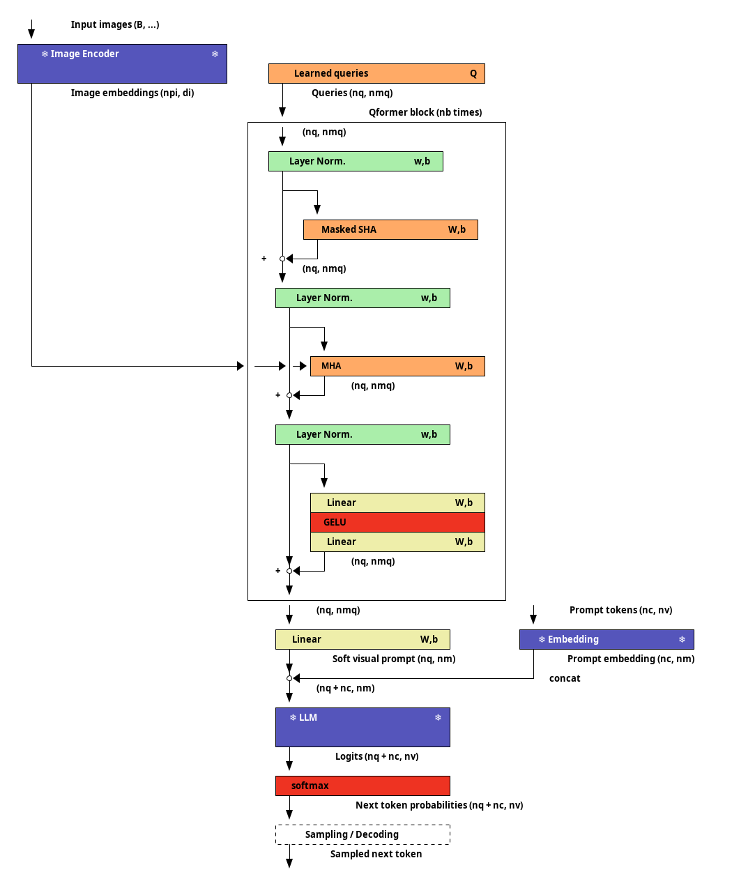
In the second stage of pre-training, the Qformer is plugged into an existing frozen LLM and must learn to adapt the information from the visual encoder to visual tokens (soft visual prompt) understood by the LLM.
LLaVA
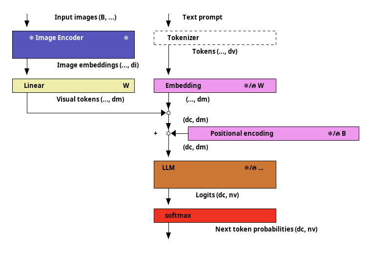
LLaVA uses a simple linear layer for projecting the visual patches (coming from a frozen image encoder) into the LLM token feature space. In the first stage (pre-training), only this small layer is trained (both vision encoder and LLM are frozen). In the second stage (fine tuning), both the linear adapter and the LLM are fine-tuned while the visual encoder stay frozen.
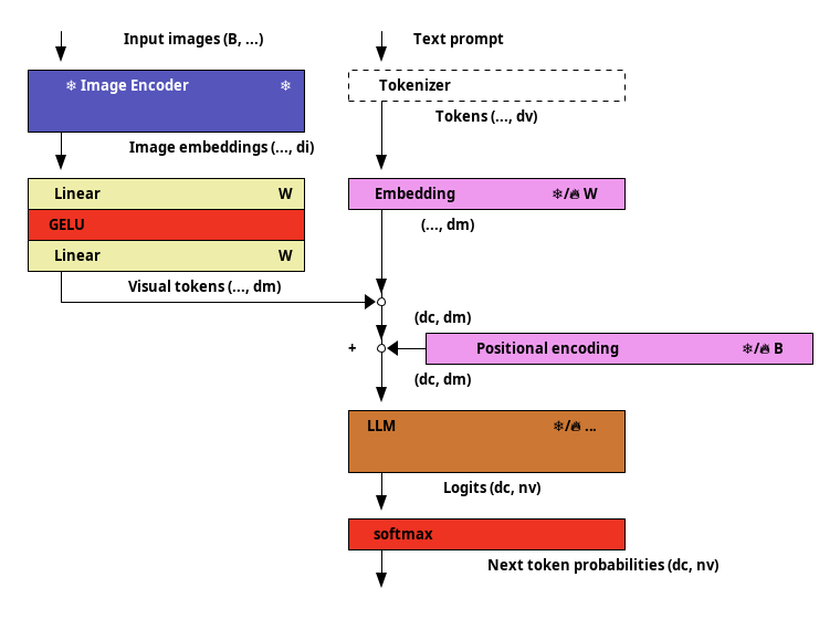
LLaVA 1.5 uses a (still very simple) FFN/MLP instead of the plain linear adapter.
PaliGemma has basically the same architecture as LLaVA 1.0 but use Prefix-LM masking: is allows non causal communication for the prefix (prompt and image tokens) but the suffix (text output) is causal. The pre-training process is different as well.
Decision models
CLM
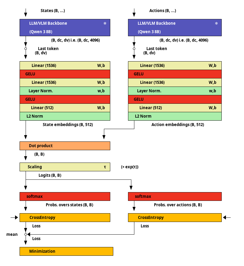
CLM is basically CLIP applied to state/action pairs with a frozen LLM instead of the image encoder and a deep projection network. After some pre-training, it is used a zero-shot action classifier.
This diagram represent the first pre-training phase (contrastive pre-training). After, that the model is also trained to distinguish the correct action among a selection of possible choices (synthetic hard negatives).
Appendix, mathematical formulas
Attention
Unscaled dot-product attention formula:
Note: dot-product attention explained
This is best explained for a single query vector
We have a sequence of keys
The query vector
Similar to many RAG systems, the dot product similarity is used to measure the similarity between
These scores (logits) are mapped to non-negative weights (
The attention uses these
In practice, we have several query vectors
The attention formula can be extended for multiple queries:
where
Example: dot-product attention
Lets take 3 key-value pairs
The scores (logits) are computed as the dot product between
We take the exponential and normalize the values to obtain the attention weights:
The result is the weighted sum of the values:
When using multiple queries, each query
For example for queries:
We have:
Each row
The attention logits are given by:
The value
The attention weights are obtained by normalizing each row:
Each row
The attentions results are computed as weighted sums of the values
Scaled dot-product attention formula:
with
Dot-product attention with QK-Norm normalizes the query and key vectors using L2 norm:
where
Generalized attention formula:
where
Masked attention
In causal (masked) attention, a given position can attend only to itself and to the previous positions. I cannot attend to future positions. Mathematically, this masking operation can be seen as setting the logits of future position to
with
producing a (lower) triangular attention matrix after the
SHA
A single-head attention layer (SHA) projects the input feature vectors (
MHA
A multi-head attention layer (MHA) is composed of several independent attention heads, each projecting the input feature vectors (
and the output of the different heads are concatenated before the output projection,
MLA
In Multi-head Latent Attention (MLA), the inputs are (down) projected (compressed) into a latent space:
These projections are then up projected (decompressed) using different parameters per attention head:
and the rest is as usual:
But instead of caching the keys and values (
Note: optimization, Q/K absorption
At inference, we can absorb the Q and K up-projections (
The attention logits (
So when computing the attention for a query
We can compute
Note: optimization, V/O absorption
At inference, we can absorb the V up projections with the output projection as well (
We have:
Which gives:
We can apply the attention in the latent space (
Deformable attention
Multi-head Deformable attention module:
with
Residual
Residual blocks have the following structure:
where
x is the identity branch (or skip branch);f(x) the residual branch (or residual update).
Token embedding
The tokens embedding layer projects tokens into the model feature space. Assuming that the input tokens
In GPT-2, positional encoding is done at this stage by adding a learned positional biases:
Token unembedding projects back the final token representations into the vocabulary space, producing token logits. GPT-2 uses tied unembedding i.e. the unembedding parameters are shared with the embedding parameters:
Recent LLM use untied unmebedding i.e.
Transformer blocks
A GPT-2 transformer block is:
A more recent transformer block is typically:
A MoE architecture:
Position encoding
In relative position bias (RPB), as attention bias
In Swin, we have 2D RPB:
where
Alternatively, RPB can use a fixed function for
FFN
In GPT-2, the FFN is:
Recent LLMs typically use a FFN module based on SwiGLU (Swish Gated Linear Unit) and without bias:
Gemma models use GEGLU (Gaussian Error Gated Linear Unit) FFN:
Normalization
LayerNorm:
where
GroupNorm:
RMSNorm:
In LLMs/Transformers, each position is normalized independently.
In convolutional networks (CNNs), normalization is done across the whole image:
where
Appendix, diagram notations
Learned parameters are represented at the right of each layer:
- greek letters for scalar;
- lowercase for vectors;
- uppercase for matrices.
Examples:
- W for weight matrices;
- w for weight vectors;
- b for bias vectors;
- B for bias matrices (eg. one bias vector per position);
- W.W for factored weight matrices;
- Q for query matrices (i.e. multiple learned queries).
Tensor dimensions are indicated in parentheses:
- ex:
(ds, dm); ds, source sequence lengthdt, target sequence lengthdc, sequence (context) lengthdv, vocabulary sizedk, number of key/query dimensionsdm, number of model featuresdh, number of features in the hidden layers of a MLPdo, number of feature of the model outputH, image heightW, image widthh, downscaled image heightw, downscaled image widthKnumber of classes (classification)Bbatch size (when relevant)
Ohter hyper-parameters:
nh, number of attention headsng, number of attention groups
References
Transformers:
- Attention Is All You Need, Vaswani et al, 2017
- The Annotated Transformer
- BERT: Pre-training of Deep Bidirectional Transformers for Language Understanding, Devlin et al, 2018 (BERT)
- Perceiver: General Perception with Iterative Attention, Jaegle et al, 2021
- A Mathematical Framework for Transformer Circuits
Autoregressive LLMs:
- Improving Language Understanding by Generative Pre-Training, Radfort et al, 2018 (GPT-1)
- GTP-2
- Official GPT-2 source
- Language Models are Unsupervised Multitask Learners, Radford et al, 2019 (GPT-2)
- Llama 3
- The Llama 3 Herd of Models, Llama Team, 2024
- Llama 3 codeSu et al, 2021 (RoPE)
- DeepSeek:
- DeepSeek-V2: A Strong, Economical, and Efficient Mixture-of-Experts Language Model, DeepSeek-AI, 2024 (MLA)
- DeepSeekMoE: Towards Ultimate Expert Specialization in Mixture-of-Experts Language Models, Dai et al, 2024
- DeepSeek-V3.2: Pushing the Frontier of Open Large Language Models, 2025 (DSA)
- DeepSeek-R1: Incentivizing Reasoning Capability in LLMs via Reinforcement Learning, DeepSeek-AI, 2025
- DeepSeek-V4: Towards Highly Efficient Million-Token Context Intelligence, DeepSeek-AI, 2026
- PLE:
- RoFormer: Enhanced Transformer with Rotary Position Embedding, 2021
Vision models:
- An Image is Worth 16x16 Words: Transformers for Image Recognition at Scale, Dosovitskiy et al, 2020 (ViT)
- DeiT:
- Training data-efficient image transformers & distillation through attention, Touvron et al, 2020 (DeiT)
- DeiT code
- Swin Transformer: Hierarchical Vision Transformer using Shifted Windows, Lui et al, 2021 (Swin)
- DINO:
- CLIP:
- MAE:
- Masked Autoencoders Are Scalable Vision Learners, He et al., 2021 (MAE)
- Masked Autoencoders source code
- BLIP 2:
- LLaVA:
- Visual Instruction Tuning, Liu et al, 2023
- Improved Baselines with Visual Instruction Tuning, Liu et al, 2023 (LLaVA-1.5) * LLaVA website
- LLaVA code
- Flamingo: a Visual Language Model for Few-Shot Learning, Alayrac et al, 2022
- DeepSeek:
- DeepSeek LLM: Scaling Open-Source Language Models with Longtermism, DeepSeek-AI, 2024
- DeepSeek-V2: A Strong, Economical, and Efficient Mixture-of-Experts Language Model, DeepSeek-AI, 2024
- DeepSeek-V3 Technical Report, DeepSeek-AI (2024)
- DeepSeek-R1: Incentivizing Reasoning Capability in LLMs via Reinforcement Learning, DeepSeek-AI, 2025
- DeepSeek-V4: Towards Highly Efficient Million-Token Context Intelligence, DeepSeek-AI, 2026
- Better & Faster Large Language Models via Multi-token Prediction, Gloeckle et al, 2024
Detection:
- DETR:
- End-to-End Object Detection with Transformers, Carion et al, 2020 (DETR)
- Official DETR code
- Deformable DETR: Deformable Transformers for End-to-End Object Detection, Zhu et al, 2020
Segmentation:
- Per-Pixel Classification is Not All You Need for Semantic Segmentation, Cheng et al, 2021
Decision models:
Misc:
- Root Mean Square Layer Normalization, Zhang et al, 2019
- Learning Factored Representations in a Deep Mixture of Experts, Eigen et al, 2013 (MoE)
- Language Modeling with Gated Convolutional Networks, Dauphin et al, 2016
- GLU Variants Improve Transformer, Noam Shazeer, 2020
- Weight Normalization: